The eigenvalues, or "latent roots", or "characteristic roots", of a correlation matrix are sometimes used as a means of estimating the number of factors (or components) which may underpin a test, or a scale.  There are often times when researchers would like to be able to say that their test is unidimensional, involving a single factor or construct.  Some feel that a test may be said to be unidimensional if it can be shown that the largest eigenvalue underlying the test's correlation matrix is so dominant that it dwarfs the others.  (See references and discussion below.)

 

Eigenvalues are computed if the System worksheet has "yes" in Row 22, Column 2.

 

Lertap's eigenvalue extraction uses computational routines produced by Leonardo Volpi and the Foxes Group in Italy, made available by the authors' kind permission.  The Foxes Group's general matrix package, "Matrix.xla", is freely available at: http://digilander.libero.it/foxes/index.htm.  Matrix.xla is a powerful, extensive set of matrix manipulation routines for use with Excel; it includes the ability to produce a complete principal factors / components analysis, with Varimax rotation, something Lertap users may wish to experiment with.

 

Here's a sample of Lertap's output with "eigens":

 

 

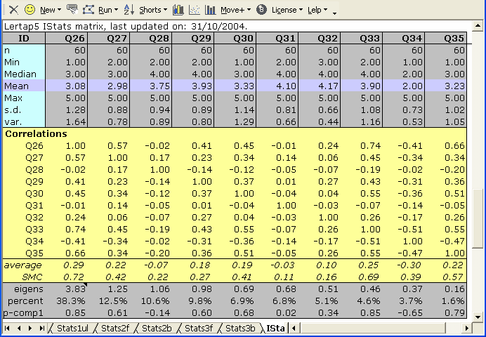
In this example, the 10-item "Comfort" affective scale seen in the Lertap Quiz data set, the largest eigenvalue was 3.83, the smallest 0.16.  In a well-conditioned correlation matrix with 1's (ones) on the diagonal, the sum of the eigenvalues will equal n, the number of test items (assuming the correlations are Pearson product-moments, not tetrachorics).

 

The row with the actual eigenvalues is followed by the "percent" row seen above.  The percent figures appear whenever the correlation matrix has 1's on its diagonal; when the SMC setting is on, and SMCs are found on the diagonal, two changes are made to the table: the percent figures are not created, and the correlations found in the p-comp1 row are replaced with correlations between the item and the first principal factor, with the row's label then changing to p-fact1.

 

What do the percent values mean?  Well, first note that there are ten items in this example, Q26 through Q35.  There are also ten eigenvalues.  As noted above, the sum of the eigenvalues equals the number of items: 10 in this example.  The percent value for the first eigenvalue is 100(3.83/10), or 38.3%.

 

Each eigenvalue corresponds to what's called a "principal component".  If we could look at the multivariate scatterplot of the ten items, and if each item had a distribution meeting the requirements of the normal distribution, the scatterplot would have the form of an n-dimensional ellipsoid, where n is the number of items (10 in this case).  If the items are uncorrelated, the ellipsoid is an n-dimensional sphere.  If, on the other hand, the items are correlated, the sphere stretches out to an ellipsoid.

 

After the percent row comes the "p-comp1" row, giving the correlation of each of the items with the first principal component -- the values found in this row are also sometimes called the "loadings" of the items on the first principal component.

 

The first principal component corresponds to the ellipsoid's major axis, to its longest axis.  Each eigenvalue represents the relative length of one of the ellipsoid's axes.  Each of these axes is said to represent, or correspond to, a principal component.

 

Think for a moment of the case when n=3.  If the three items are normally distributed and uncorrelated, their scatterplot will have the form of a soccer ball, a perfect sphere.  As the three items begin to correlate, the soccer ball changes shape, morphing into an American football, and then, as the correlation among the items increases, into a cigar shape.  The shape of the scatterplot is highly related to the relative sizes of the eigenvalues; if the eigenvalues are all equal, the shape is a sphere.  If the first eigenvalue is much greater than the others, the shape is a cigar, and in such a case the multivariate scatterplot is said to have, essentially, one principal component, or dimension.

 

In the 10-item example above, the first principal component is said to account for 38.3% of the total variance (or volume) found in the multivariate scatterplot.  As the size of the first component comes to dwarf the others, some people say there appears to be but one dimension underlying the items, which, in turn, often leads people to say that the items are "measuring the same thing".

 

Lertap will also "plot" the item-component correlations (or loadings) in bands.  It takes the values found in the p-comps1 row, and makes a little table, such as the one below:

 

 

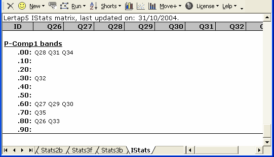
The P-Comp1 bands indicate that there's a group of six items, Q26, Q27, Q29, Q30, Q33, and Q35 with high correlations on the first principal component.  If we were to create a new subtest using just these items, chances are very good we'd end up with a coefficient alpha value much higher than that obtained for all ten original items.

 

And, speaking of alpha values, did you happen to notice that one of the eigenvalues seen above, the first one, has a little black triangle next to it?  (This triangle is really red, not black, but for some reason when we took our snapshot of the original screen the colour changed.)

 

When you have your own IStats screen showing, find one of these triangles and let your mouse hover above it.  Lertap will display the alpha value for the corresponding principal component; in this case the value turns out to be 0.821 -- it can be shown that this value, 0.821, is the maximum possible value which coefficient alpha could assume for any linear combination of the items comprising the subtest.  (Please refer to the technical paper cited below for more information, and also please note that these small triangles will appear only when the corresponding alpha value is equal to or greater than 0.60.)

 

The Scree Test / Plot

When we think about the first eigenvalue possibly "dwarfing" the others, we might well long for a picture of some type.  The scree test was invented by Cattell way back in 1966 to meet these longings.  Cattell suggested we graph the eigenvalues from highest to lowest to see if the first eigenvalue, or the first few eigenvalues, dwarf the others.  His suggestion remains popular to this day.

 

We can graph our 10 eigenvalues using a couple of methods.  The plot shown below was obtained by selecting the eigenvalues, and then using Excel's Insert / Chart (Line) options.  An easier way to accomplish much the same thing is to use an option from the Lertap tab on the Excel ribbon: there is a "Line" option in the "Basic options" icon group.

 

 

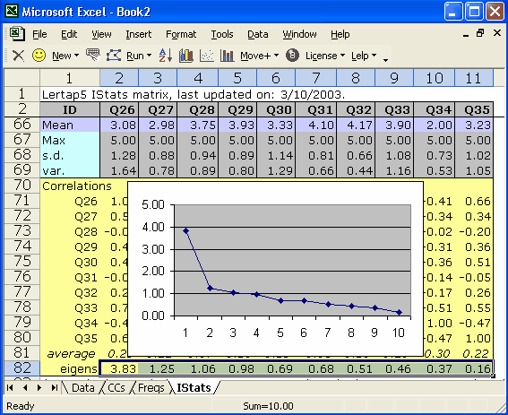
The so-called scree test for the number of factors involves nothing more than eye-balling a line graph such as the one above, and deciding where the scree begins.  In case you've forgotten, the scree is all the loose rocks at the base of the cliff your friends want to climb, those pesky fallen chunks where your boot will slip in and get stuck, twisting your ankle, granting access to a face-saving retreat to the beer tent in case you were really too chicken to climb the cliff to begin with.

 

Does the first eigenvalue dwarf the others?  Does our scree begin with the 2nd eigenvalue, or the 5th?  This question will remain unanswered here; many times the start of the scree is much easier to detect.  For references on the scree test, see Catell (1966), Pedhazur and Schmelkin (1991), or search the Internet.  

 

Note that eigenvalues can go negative.  This is likely, for example, when SMCs are used on the diagonal of the correlation matrix, when one of the items has no variance, or (especially) when tetrachoric correlations are used.  Also note that it is possible for the eigenvalue extraction method used by Lertap to fail; the method is an iterative one which concludes when the iteration process appears to converge. Under some circumstances convergence will not occur -- eigenvalues will not be returned in such cases (but it may be worthwhile to try again, that is, to return to the Run menu, click on the "More" option, and again request "Item scores and correlations").

 

The computation of eigenvalues can be a timely, labour-intensive task for your computer.  If you will not be making use of eigenvalues, and have no desire to become an avid scree plotter, then you'll want to turn off the eigenvalue option in the System worksheet (the option's setting is found in Row 22, Column 2 -- set it to "no").

 

More timely comments may be found by paging ahead to the time trials topic.

 

---

Related tidbit:

 

For more about these topics, see "Some observations on the scree plot, and on coefficient alpha", a 16-page document with lots of little tables and some wonderful screes, available via the Internet: click here if you're connected.